Fourth week
In this week, it is expected that the image and 3D cloud treatments are finished. First it was necessary to remove the noise from the depth sensor from the kinect like the next example. 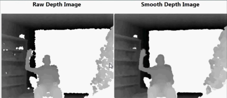
Image 1- example of a 3D image smoothing
To do so, first it was tried a function available at Link
The use of this function created another problem, some of the information was deleted.
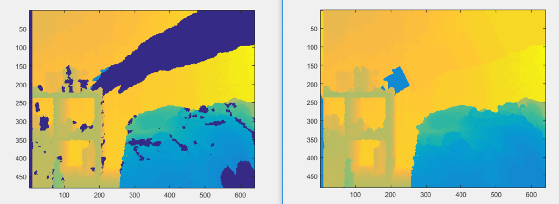
Figure 2 - Funcion kinect depth normalization
As it is possible to see on figure 2, my arm disappear in the right image as well as most of the detail. This would possible create problems by not detecting the holes on a surface or maybe confuse a surface with the background.
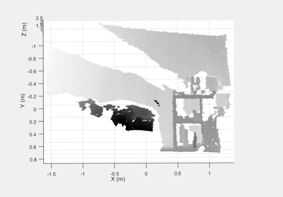
Figure 3 - Point Cloud with kinect depth normalization
As it is possible to see in figure 3, the point cloud is missing a lot of detail, almost the same as if it was not used.
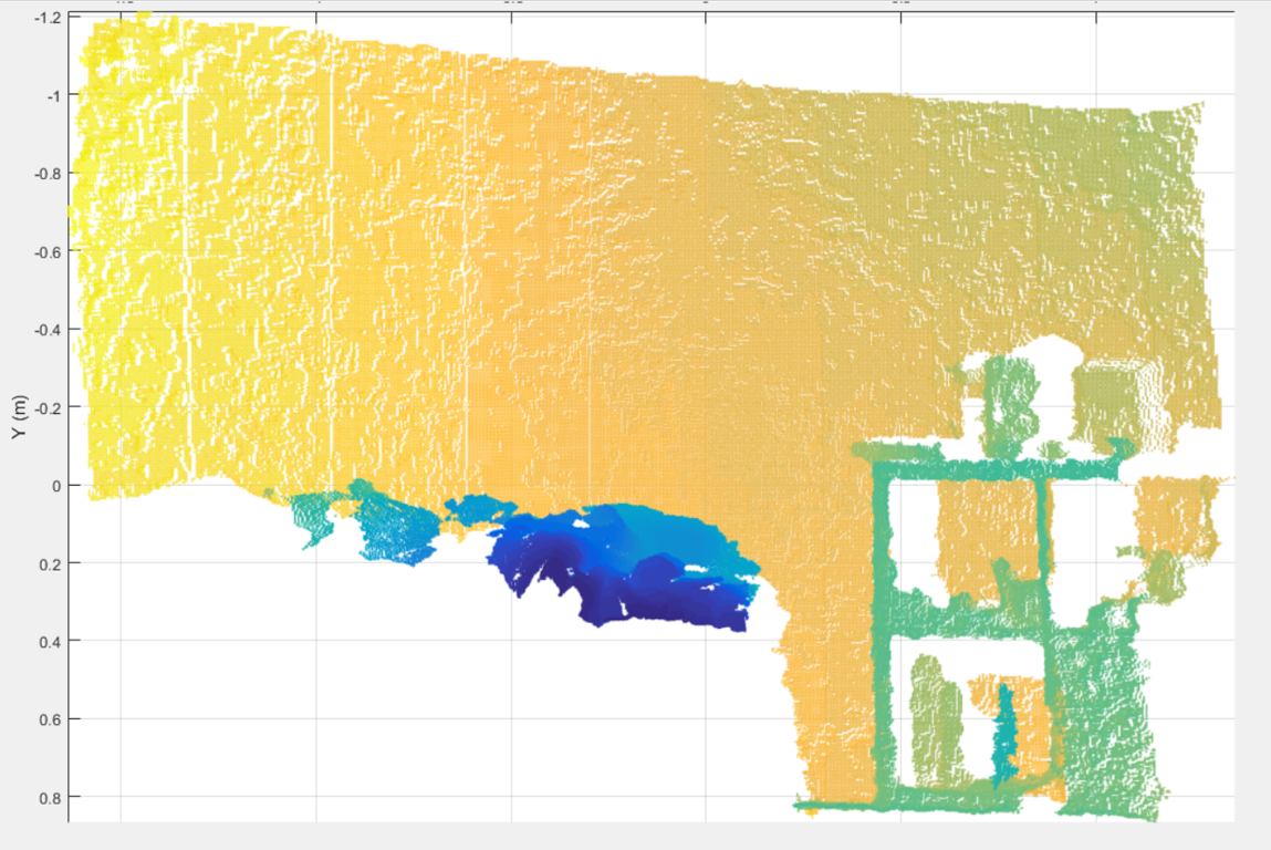
Figure 4 - Original Point cloud
The original point cloud was obtained using the tutorial that was available at mathworks at 06/03/2017 on the Link
Since the function created more problems than those it could solve, another solution was attempted. By observing the preview image of the depth video feed from the kinect, it was noticed that parts of the image would appear and disappear with time. So the solution tried was to get multiple snapshots and complete the missing information in one snapshot with the others.
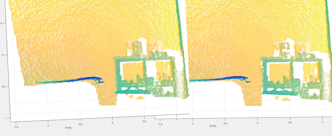 Figure 5 - Comparison between the original mesh (right) and the mesh with multiple layer (left)
As it is possible to see, the mesh on the left is more refined than the one on the right, the only inconvenient is that it takes a couple of seconds to get all the snapshots. The method used to get all the snapshot was a for cycle with a pause of some milliseconds between each, then a mask was created to read all values of 0 from the previous snapshot and replace them with values from the new if available. The replacement was done by multiplying the mask by the new snapshot. The mask was from type uint16 as well as the snapshot.
Now with the refined mesh, it is necessary to associate the depth coordinates with the 2D from the image.
The firs thing done was to remove all of the points that would not be from the intended part. This was done with the same method described before, using a mask and multiplying operations. The result is in figure 6.
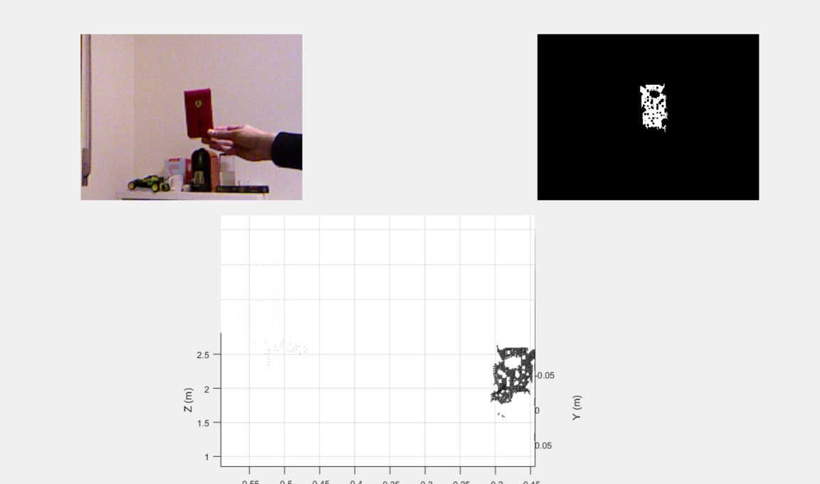 Figure 6 - Mesh treated
This was just to test the concept, so the mesh and the image with the black background, in figure 6, did not received any complex treatment, just a conversion from RGB to HSV and then the values of the H from the powerbank were chosen by trial an error.
To test it on a more controlled environment, a scene was created to simulate possible working conditions.
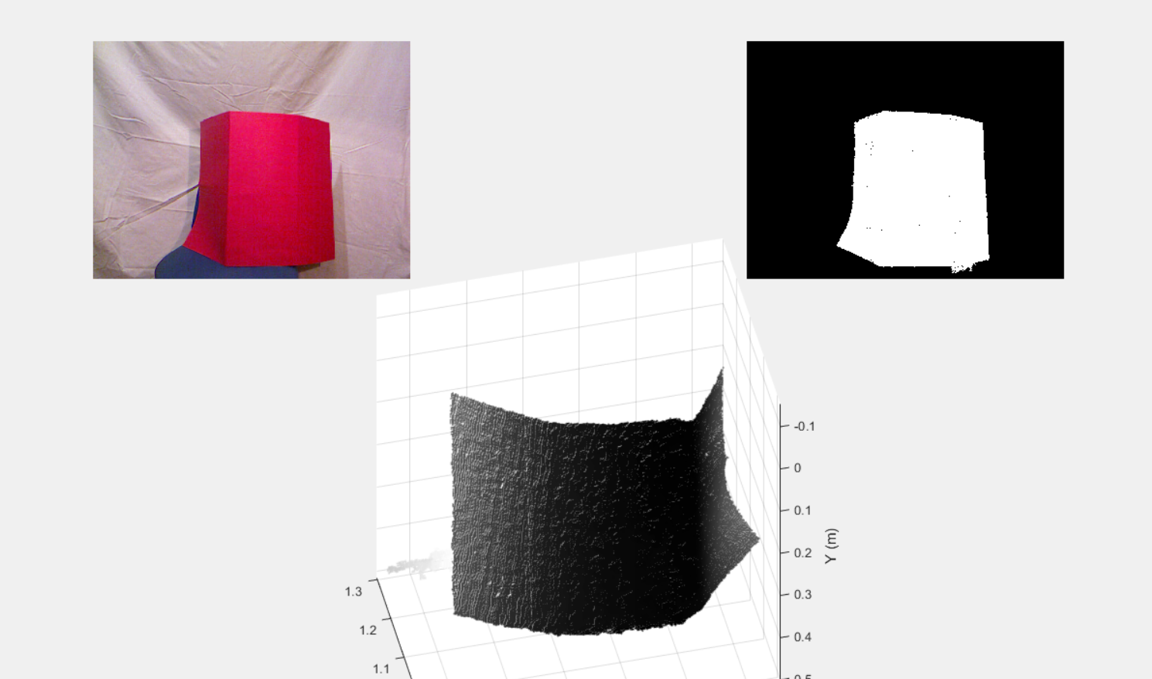 Figure 7 - Test on a "controlled environment"
In this test its possible to see the surface is much more refined, as the previous it was very hard to get the same result and it would influence the gradient calculations.
Now with this surface, the gradient was calculated so it would be possible to divide the surface in zones with same intervals of gradient. The result is in the following image.
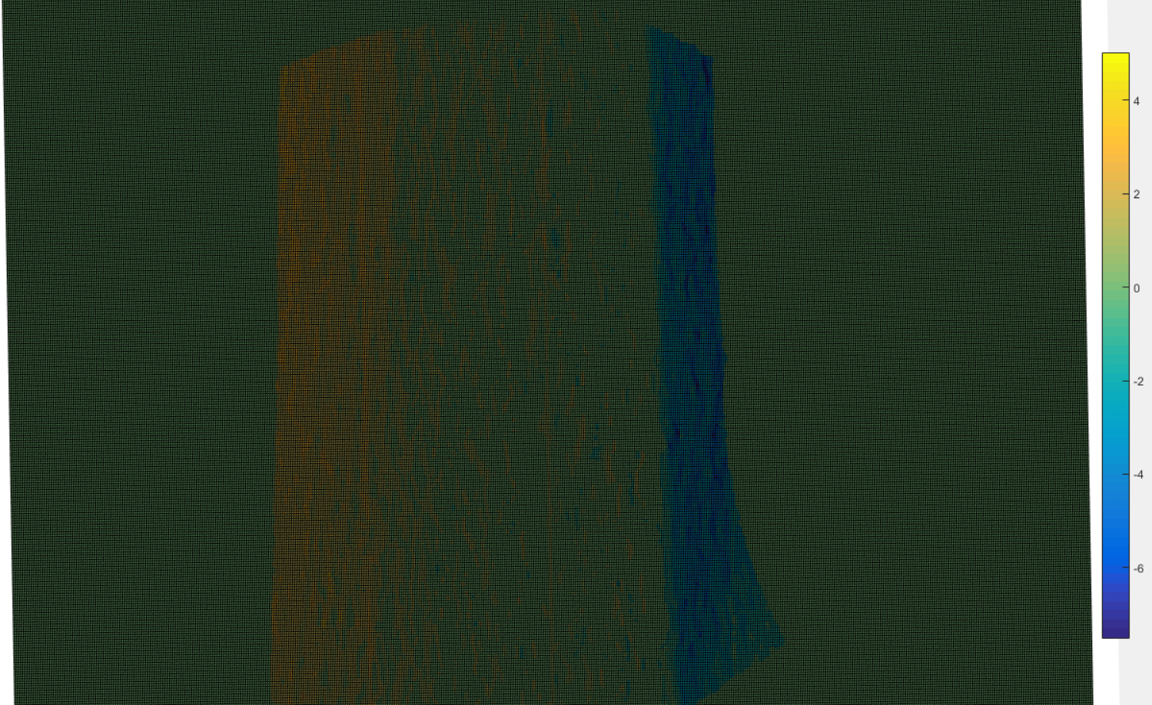
Figure 8 - Gradient calculations
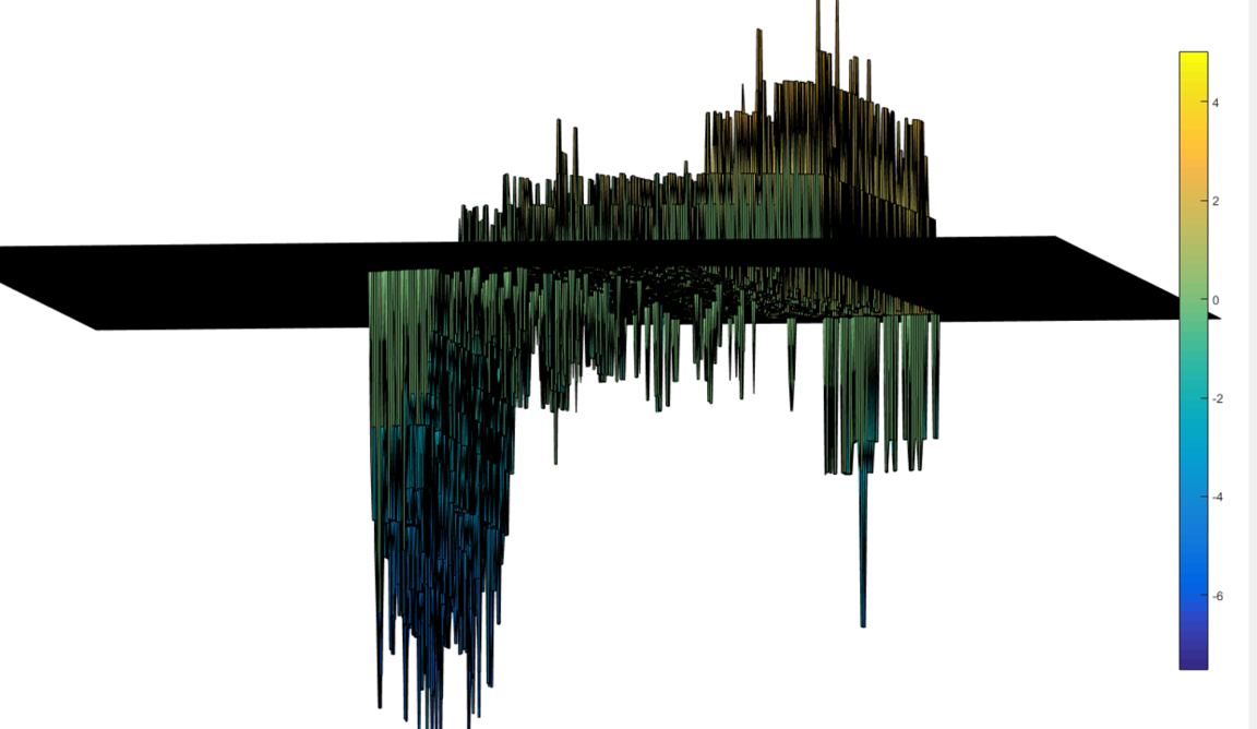
Figure 9 - Gradient Bars
As it can be seen on both images, 3 zones can be visualized. Also an median filter was used to smooth the values.
Now it is just necessary the creation on zones based on the different gradients calculated.
The idea was to use the max and min values from figure 9 and divide into a certain number of similar intervals. The first trial resulted in the figure 10.
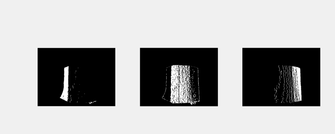 Figure 10 - Different zones
The different zones still would need treatment but it would be interesting to first developed a user interface that could change different parameters in order to get the expected results.