Twenty seventh week
So by drawing a square with the limits of the galvanometer, it was found that the x axis was smaller than the y axis. This could be a galvanometer problem if it wasn't for the potentiometer on the driver that can be adjusted.
So to adjust the the potentiometer in order to do 20º another temporary structure was build to indicate where the 20º should be.
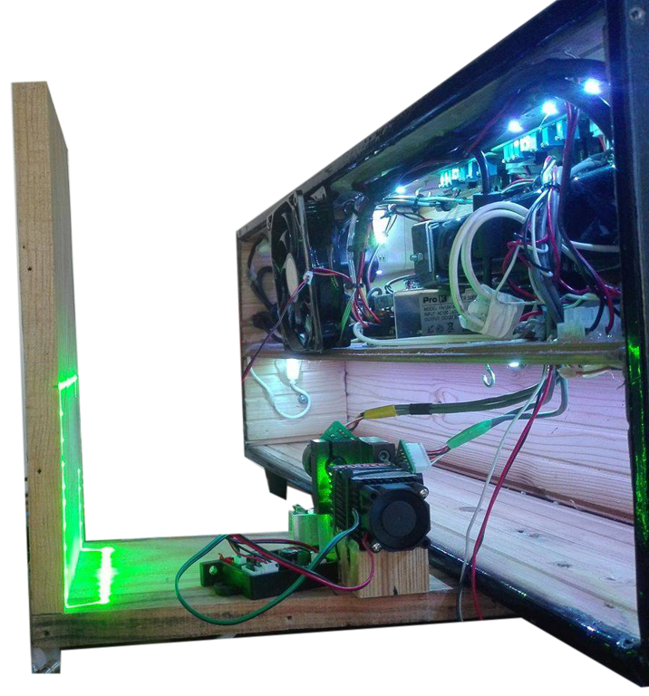
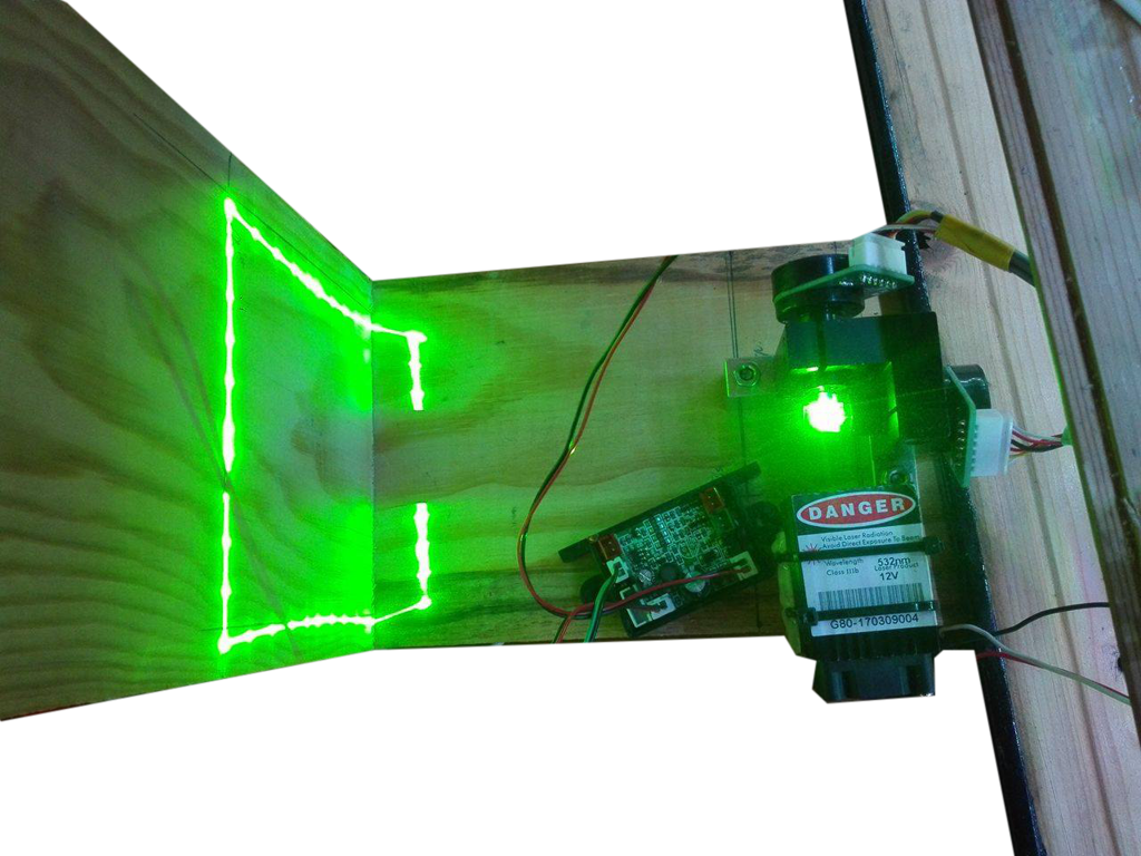
Figure 2 - Top view
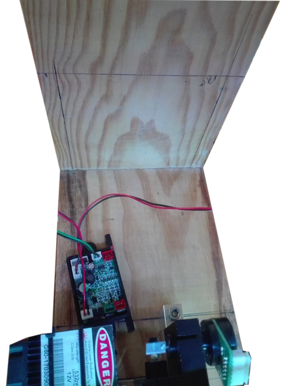
Figure 3 - Measurements on the wood to calibrate.
By performing this task, another problems arrived. The points that after this calibration were in the correct place, at least the drawing was equal to the one on the app, were now just a small line instead of a point, this means that the laser is turning on when the galvanometer is still trying to reach the correct coordinate.
After a quick research, it was found that there are a couple of other different variables that needed to be adjusted. Since there is no information on how to calibrate the drivers, this task can't be done, since the drivers need someone with knowledge on this kind of calibrations.
This will be the only topic missing, but, with a calibrated galvanometer, everything that was built and programmed, should work the it.
This way the writing of the thesis will continue.
Twenty sixth week
This way the problems with the address of the DAC's were solved. So the construction of the shield begun. It needs to have the same functions in the same pins as the low pass filter shield so the shields could be replaced without the need to change the arduino code.
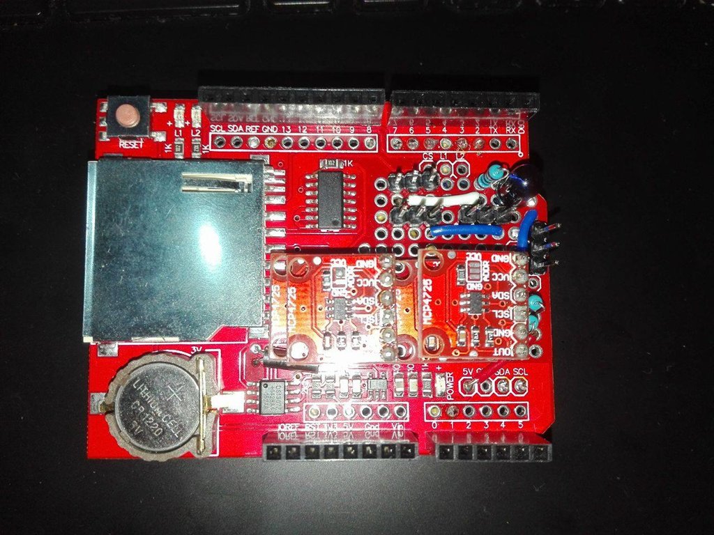
Figure 1 - Top view Shield
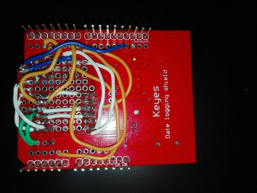
Figure 2 - Underneath view of the shield
The arduino code for the dacs was also built. Leaving only the calibrations to do.
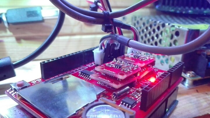
Figure 3 - DAC shield connections.
The purpose of the figure 3 is to show the position of the 2 galvanometer wires are connected for future reference.
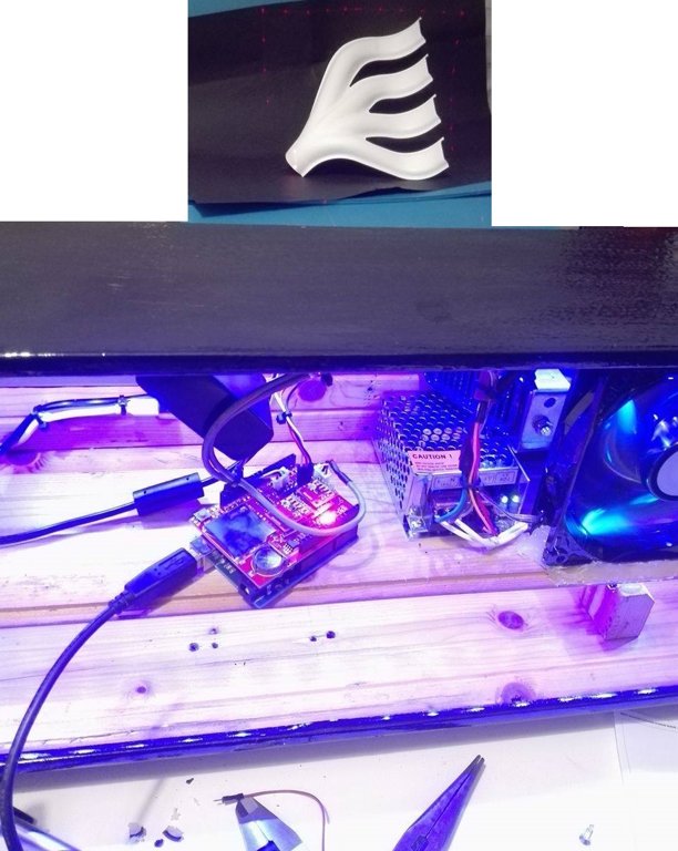
Figure 4 - Using the DAC shield to do a square with the galvanometer limits
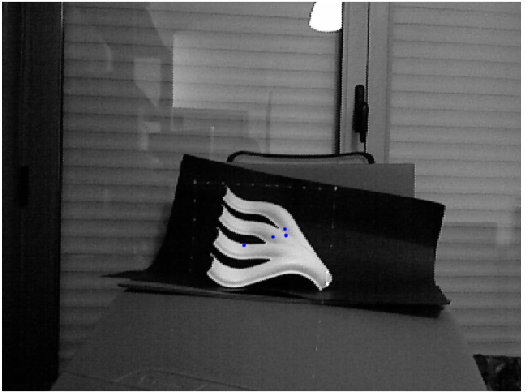
Figure 5 - Mesh points on the computer
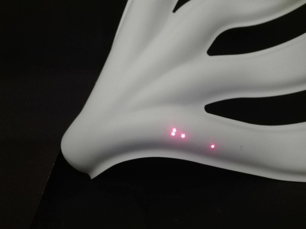
Figure 6 - Result on the object
As said before only the calibrations are missing right now.
As for the green laser pointer, it can use 12v or 5v. Using the 5V from the arduino, the laser has trouble flashing with the same speed as the red pointer. When the laser is connected to the 12v, the bright is super intense, and can cause harm by looking at his reflections. The green laser is class III b. This way the laser that will be used is the red one. This can be changed any time just by removing the red and connecting the green laser, since there is no changes in the code.
Twenty fourth to Twenty fifth weeks
- Time to write 40 points (square) without delays - 1812 microseconds;
- Max number of points of the galvanometer - 20 000 points per second;
- Points to get 20 frames - 1000 points (20 000/20) ;
- To represent something 20 times per second means 1000 points in 50 ms;
- Delay according to the number of points - 1000 points in 50 ms, means 1 point with a delay of 50 microseconds.
Tests with the arduino showed that the galvanometer can't handle that speed, instead the pause was 140 microseconds. The figure used to test it was a square with 10 points in each side. Then, by turning the laser on after the 140 microseconds delay, it was observed that it was on before the galvanometer reached it's destination. So in order to turn on the laser when the location of the mirrors was the intended point, the necessary delay was 700 microseconds. Then, for the laser to be seen it would need a delay of 50 microseconds. The final delay is 750 microseconds. with means that only 66 points will be possible at 20fps.
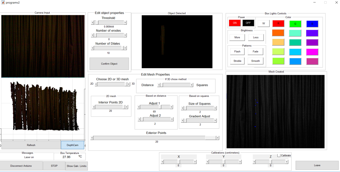 Figure 1 - New app ( the calibrations panel still needs work)
The new app allows to:
- Control the box lights;
- See the box temperature;
- View the point cloud in real time from the kinect; ( it's possible to hide it and see the depth cam image instead.)
- Show the galvanometer limits to show the user, where to put the part.
To change the colour of the box lights, infrared communication between the arduino and the lights (bought with the receiver) was established. 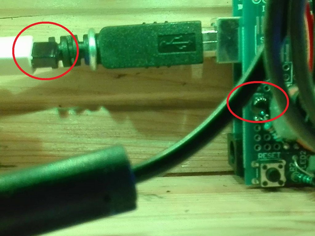
Figure 2- IR sensors
To read the temperature, a temperature sensor was installed on the top of the second shelf. Since the drivers of the galvanometer, when "online", heated up to a reasonable temperature, a fan was installed. The fan speed is always maximum since its connected directly to the 12V power source. The decision to keep it that way was the lack of time.
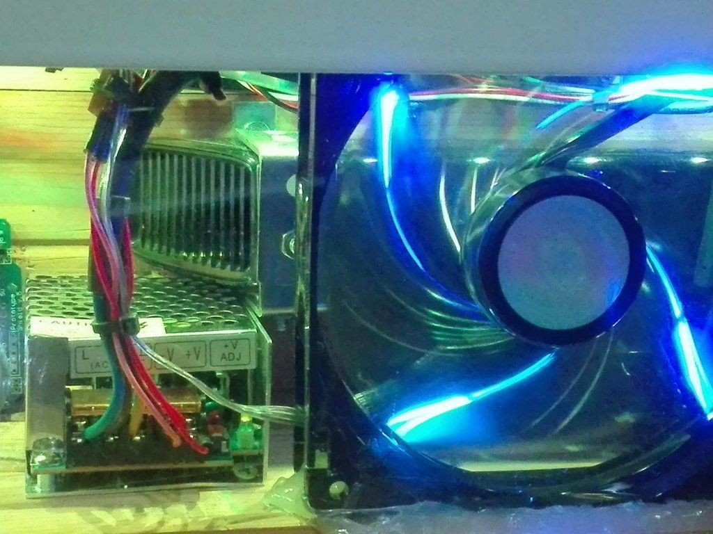 Figure 3 - Fan and 12V power source
To work the the serial port, more code on the matlab and arduino was developed.
One timer was created on the arduino to send the temperature every 2 seconds and another two were created on the matlab for the app, one to update the point cloud every 250 milliseconds and another to look for COM ports available.
The code for the arduino to recieve the data of the points was rewritten. The readuntilstring() function, when used to read large strings fails. So an alternative function used to read the string char by char and build the string. Then getValue() was used, which was found on link, separates the string in smaller strings by the char ";", which was the same used before. Since the entire string was saved, no need to create a matrix to save it, so that part was deleted and instead of readding a matrix, the string will be read.
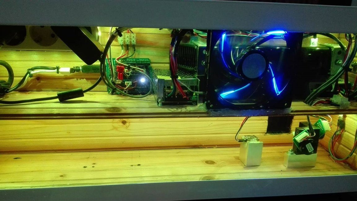
Figure 4- Box aspect inside at this date.
To avoid having 3 wires laying around, a solution with a usb hub and a usb extension cable was studied but the kinect somehow detects when it's not connected directly to the computer, so that solution was left behind.
Also, to try to only use one low-pass-filter for each mirror, a solution with a logical gate was tested, but it was found that the logical gate only works at 100% with a digital signal. So, two more low pass filters were built into the arduino shield, since the logical gate was already welded. This way, 2 pwm signal are sent, and 4 digital signals control each one of the gates. The pwm signal is sent to both pins on each mirror (up and down), and, other arduino pin controls if it is on or off.
Results.
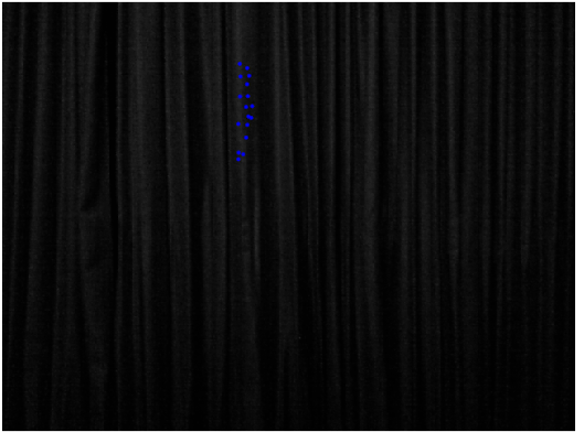
Figure 5 - Computer plot ( intended points)
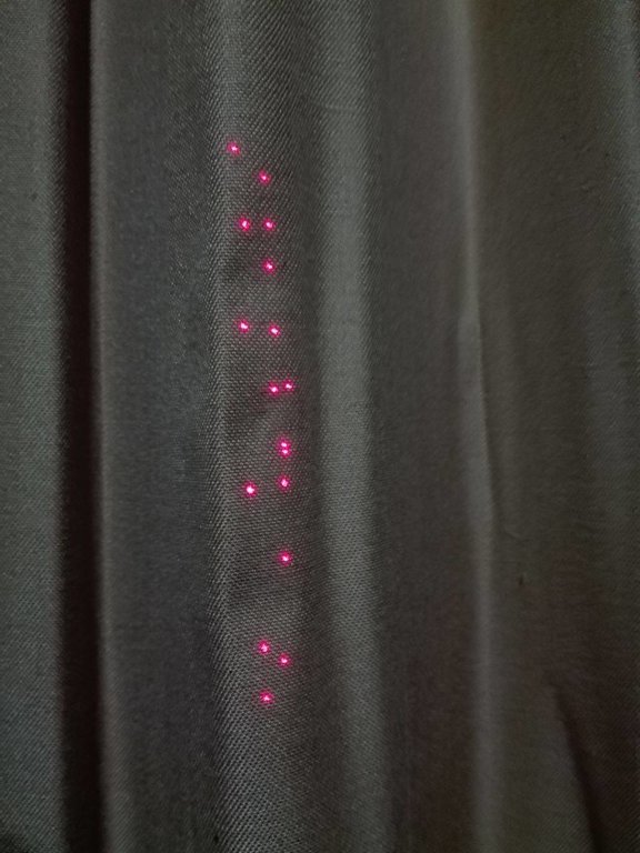
Figure 6 - Real world result
Since the old platform to hold the laser was made for the first points, its dimensions were wrong, so a new platform was built in wood for the both laser pointers, the 5mw and the 80 mw lasers.
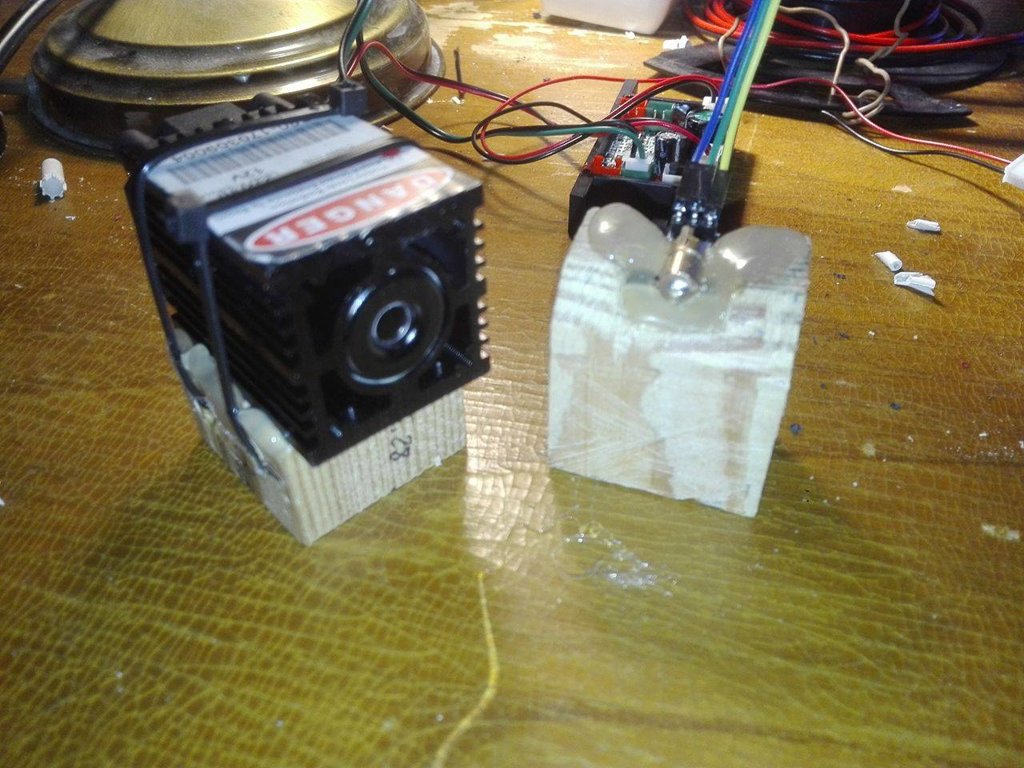 Figure 7 - Laser platforms
Also, for the vision component, a light was installed on the front of the box. Since there was no relay available at the time, a button was also installed.
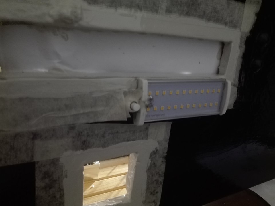
Figure 8- LED light and button
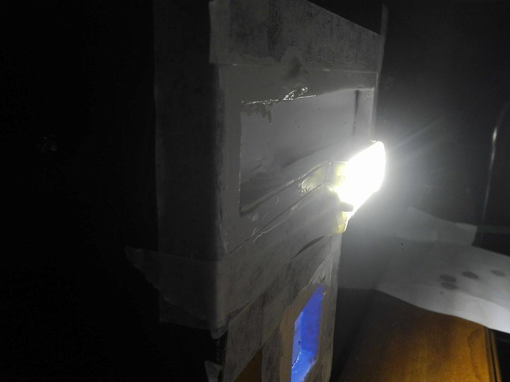
Figure 9 - LED light on
The light is positioned right under the rgb cam of the kinect.
DAC experiments
The dac that will be used on the work are the MCP4725. This device communicates via I2C. This kind of communication is made using the address of each device. Since the DAC's have the same address it's impossible to send commands to just one. So, ways to change the address have been searched. A solution was found on link which said "To change the address of your other device, simply de-solder the jumper and add a blob of solder to the middle pad and the Vcc pad."
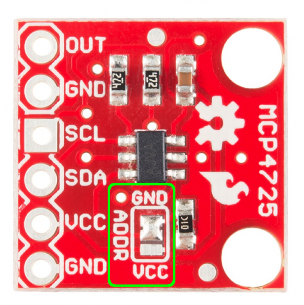
This way the addresses 0x62 and 0x63 were possible. Since only 2 DAC's were necessary at a time, the vcc pin was set to 0v on 2 DAC's and 5 on the other 2. This was supposed to allow to operate one DAC at a time but instead the system froze.
Twenty first week to Twenty third
- Creation of the equipment box.
- Creation of the shield
- Assemble of all equipment.


Figure 1-4. Equipment Box Figure 5 - Arduino Shield for low-pass-filter pwm signal
Eleventh to Twentieth week
Tests with the high frequency PWM signal have been done in order to validate the possibility of avoiding an analogue signal.
In the tests with a frequency arround 30kHz PWM, a delay of one millisecond was used for allowing the figure to be visible. With this delay and the high frequency PWM, after just 10 points, adding more would result in the impossibility of they being represented at the same time. Also, and this was the biggest issue, the laser path would have some inconsistencies, since it had the same effect as if it was being turned on and off. The first attempt to solve this issue, was a low pass filter, but the effect was the same as high frequency PWM alone.
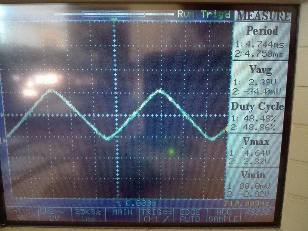
Figure 1- Result with the low pass filter, analogue write loop cycle from 0 to 255 and 255 to 0.
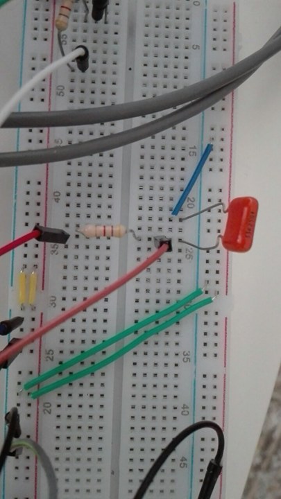 Figure 2 - Low pass filter used
The filter was used with a pwm frequency of 200kHz.
Manual work:
- Laser pointer was glued to the base.
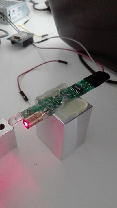 Figure 3 - Glued laser pointer
- Galvanometer was screwed to the base.
Since the laser pointer on figure 3 stopped running, another one was bought. All the problems with the galvanometer part were solved with this exchange.
Then to test the laser a figure was drawed.
 Figure 4 - Pikachu figure
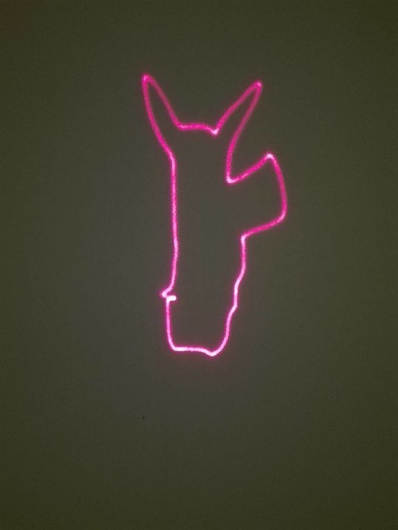
Figure 5 - Pikachu contours with the galvanometer
There is a problem with the leg of the pikachu but its possible that this problem was created when the coordinates of the leg were being copied to the arduino, since the rest of the shadow is ok. The image looks different from the figure 4 because of the scale.
Tenth week
Also, since the parts were now close to white, the background was now black. The other way around was study but the shadows produced by the parts, usually lead to some confusion by the camera, and the problem was even worst in case of small holes.
The colours tested for the background were red, pink, black and white.
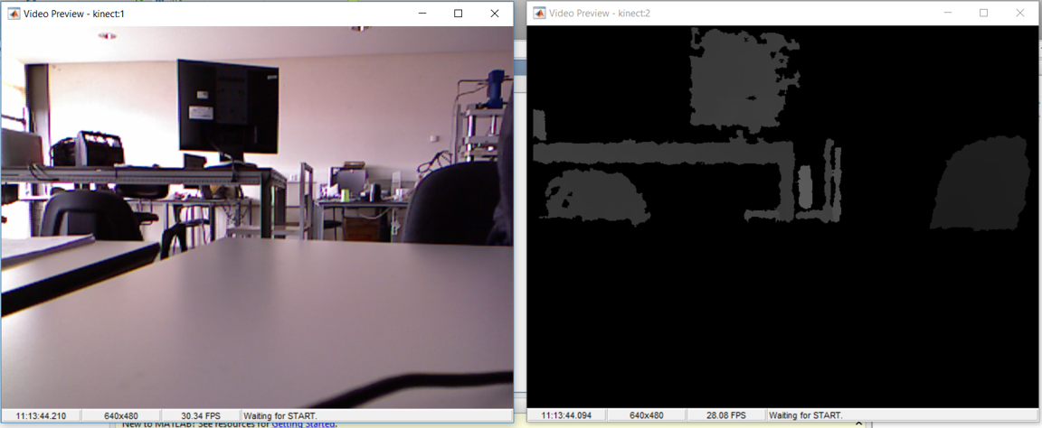
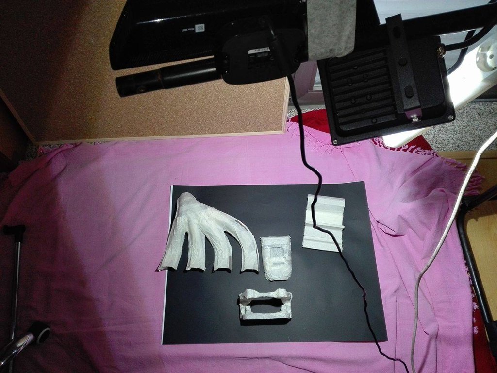 Figure 1 - Environment and object for tests
By testing the objects on figure 1, it was found that in previous tests, camera calibrations between infra-red and rgb sensors were forgotten. This problem is now corrected. To test the functions available to new matlab versions, version R2017a sponsored by Engenius - UA Formula Student was used.
Them, with the calibrations, the two methods used before were refined based on the expected result for the objects on figure 1.
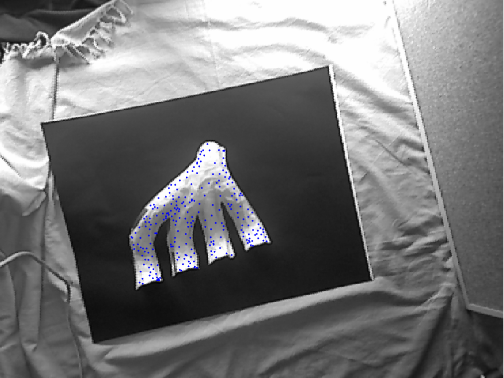 Figure 2 - Result with distance
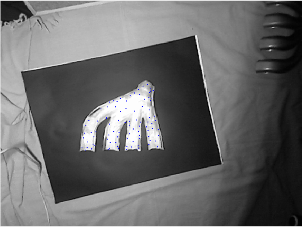
Figure 3 - Result with squares
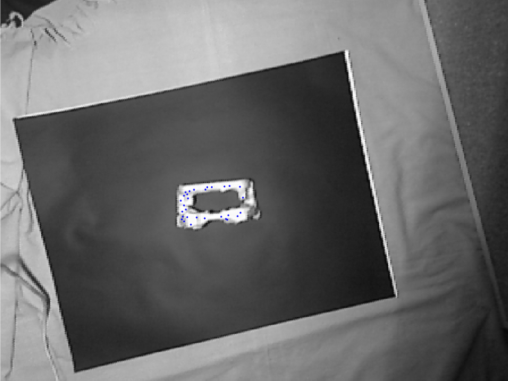 Figure 4 - Result with distance
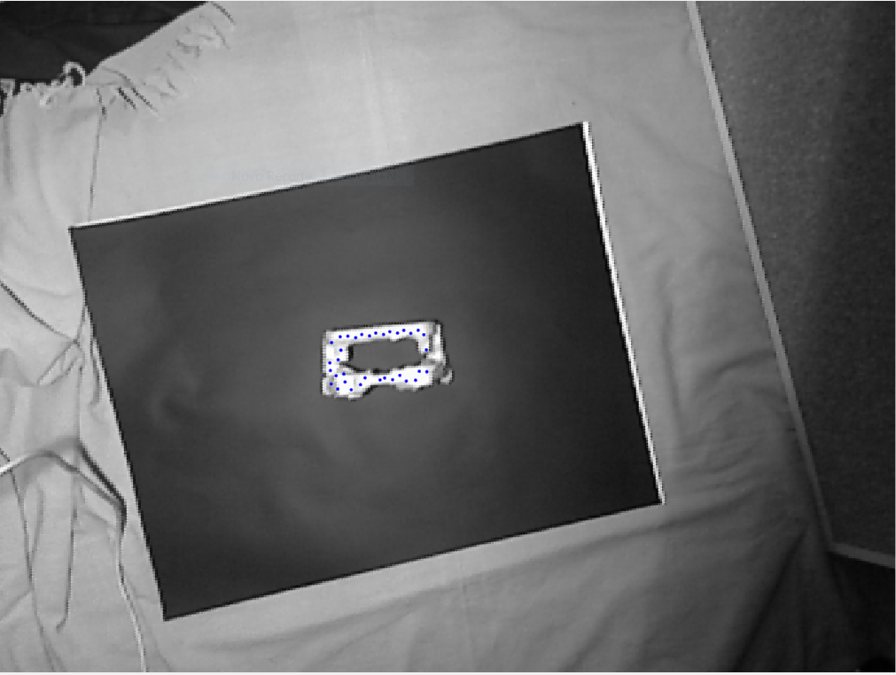
Figure 5 - Result with squares
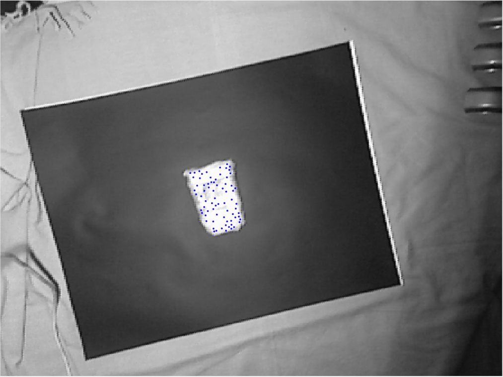
Figure 6 - Result with distance
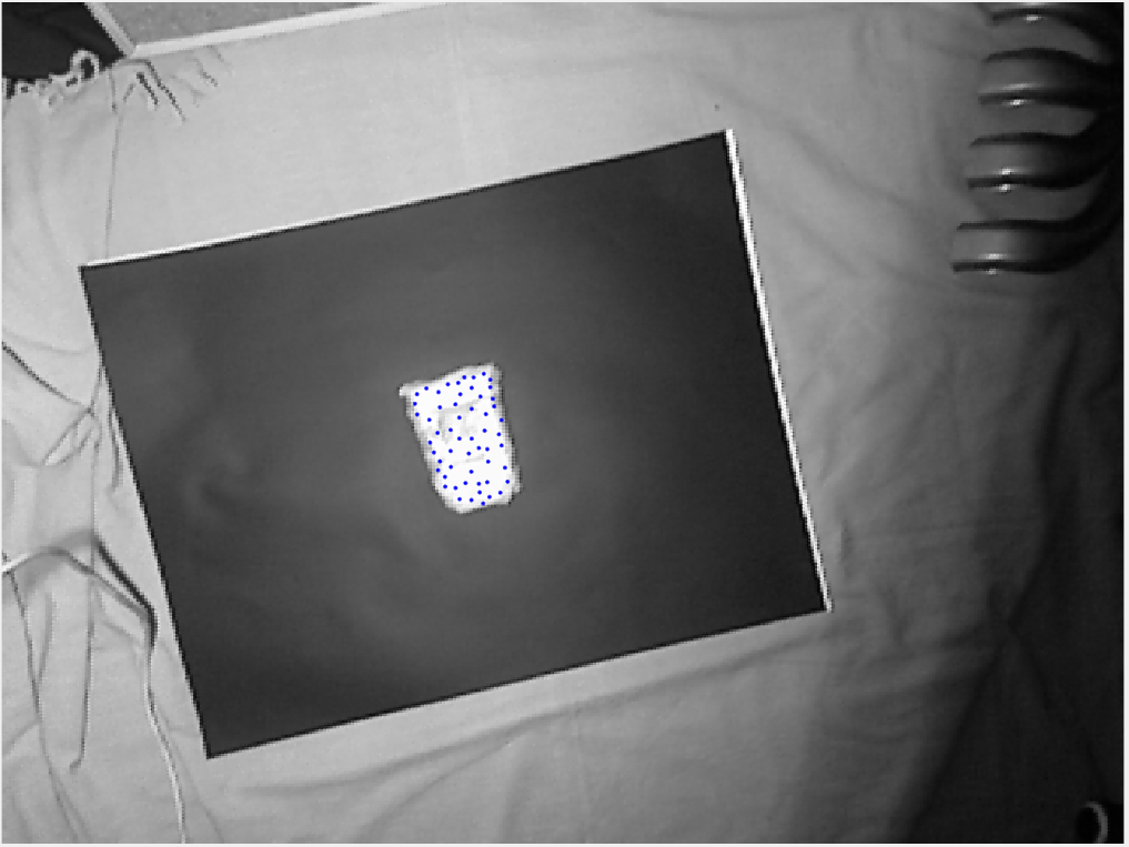
Figure 7 - Result with squares
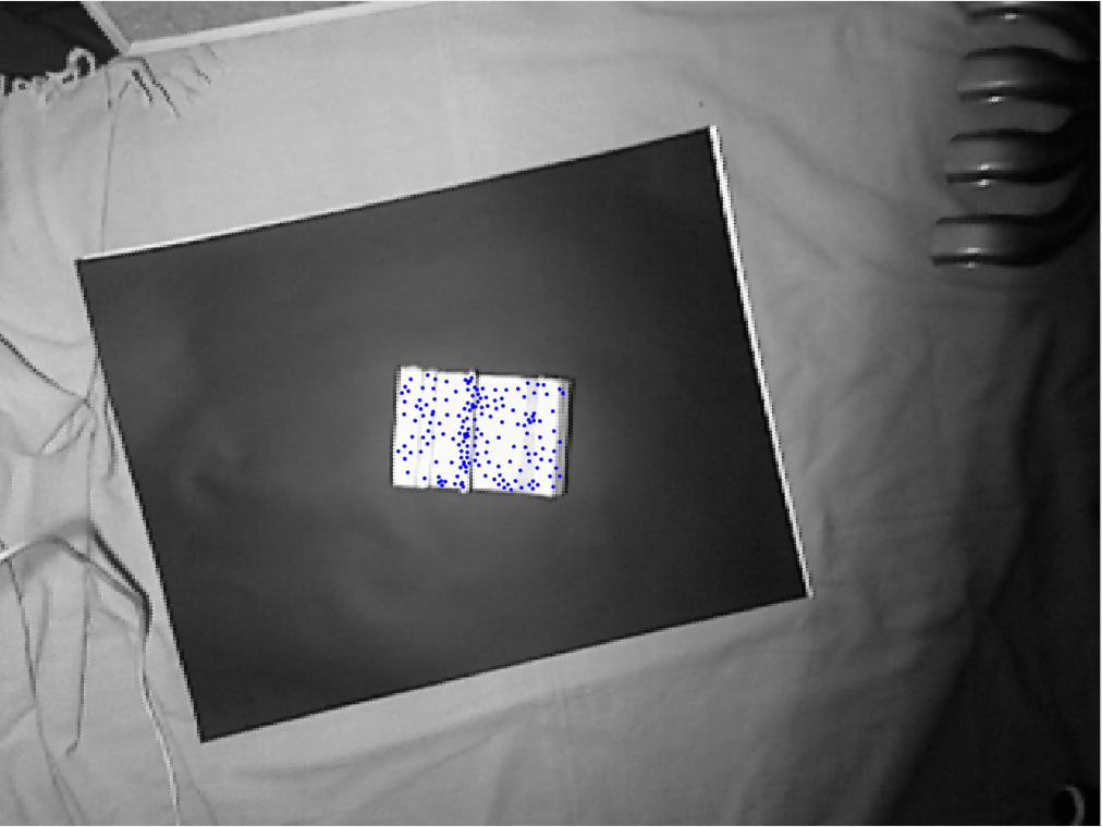
Figure 8 - Result with distance
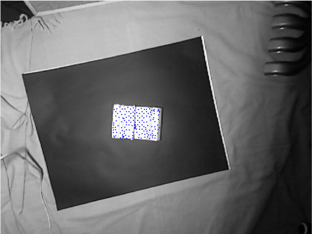
Figure 9 - Result with squares
By studding the digital potentiometer, it was found that it works in steps.
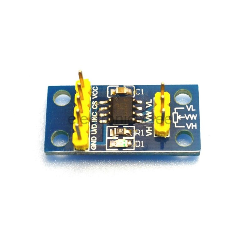 Figure 10 - Digital potentiometer
As it can be seen on the figure above the digital potentiometer has 8 pins. The Vcc and VL are connected to 5V and the GND and VH are connected do ground. The VW is the pin with the intended voltage to control the mirrors on the galvanometer.
To ensure that voltage, pins U/D (up, down), INC (increment) and CS (chip select) need to be controlled.
So, to add one step, CS needs to be low, U/D need to be high and then INC is "pressed" to increment one step by setting it to low.
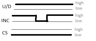 Figure 11 - Add one step to the digital potentiometer
To subtract one step, CS is still low but now U/D needs to be low, then you send low on INC
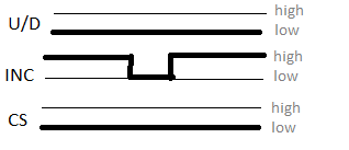
Figure 12 - Subtract one step to the digital potentiometer
To store the wiper value for the next time the device is turned on, U/D and INC both need to be high and then you set CS high.
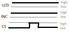 Figure 13 - Save value for the next time the device is turned on
If the CS value is high in any of the previous control steps, nothing happens because the device enters standby low power mode. The information on how the digital potentiometer works was found here youtube link.
The problem with the use of the potentiometer is that it can only get a certain number of values, that are available on the file valores.txt. To get all the values between 0 and 5 V a DAC could be used instead of the digital potentiometer.
Also it seems to be impossible to create a well visible mesh with the galvanometer, tests with the device showed that the trail created by the laser made it seem just one line. If a small delay is set between each step, for 18 points a 4ms delay it too much but 3 ms produces a blurred line.
To finish, the laser pointer used, after approx. 5 meters starts to leave a giant but since the kinect limitations are 4m it is ok.
Ninth week
With the tutorials completed, the galvanometer and the digital potentiometer were tested.
The digital potentiometer it the X9C103S but the tutorial found to the X9C103P had the same connections. Link to the turorial.

Figure 1 - How the digital potentiometer was connected

Figure 2 - Galvanometer response from 0V to 5V
Since only one digital potentiometer was given to be tested, both mirrors were set to the same movement.
One thing that was noticed was that all of the connections required a lot of wires which can get confused, a better solution would possibly be to print a circuit board to connect both potentiometer to each mirror controller.

Figure 3 - Connections with one potentiometer
All the parts were cold even if they were turned on for some hours.
Also, there is still the need to change the voltage from 0V - 5V to -5V - 5V.
Eighth week
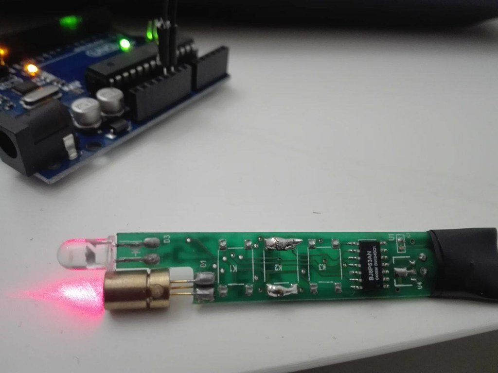 Figure 1 - Welded laser
Also the app was finished, at least the mesh creation part.
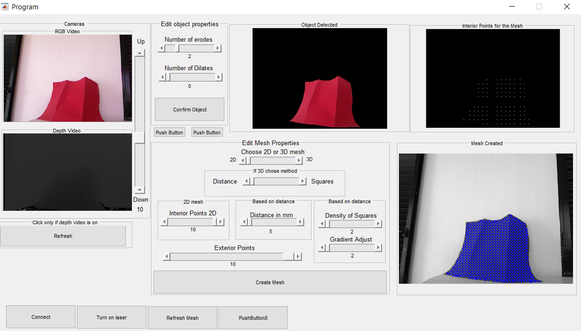 Figure 2 - Mesh using 2D
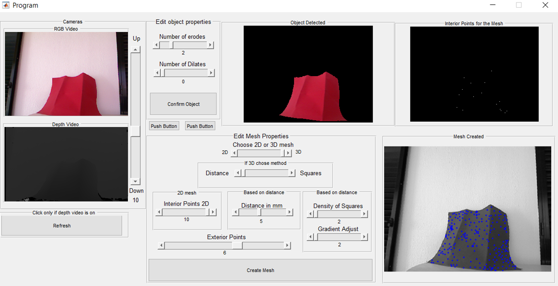 Figure 3 - Mesh using distance between points
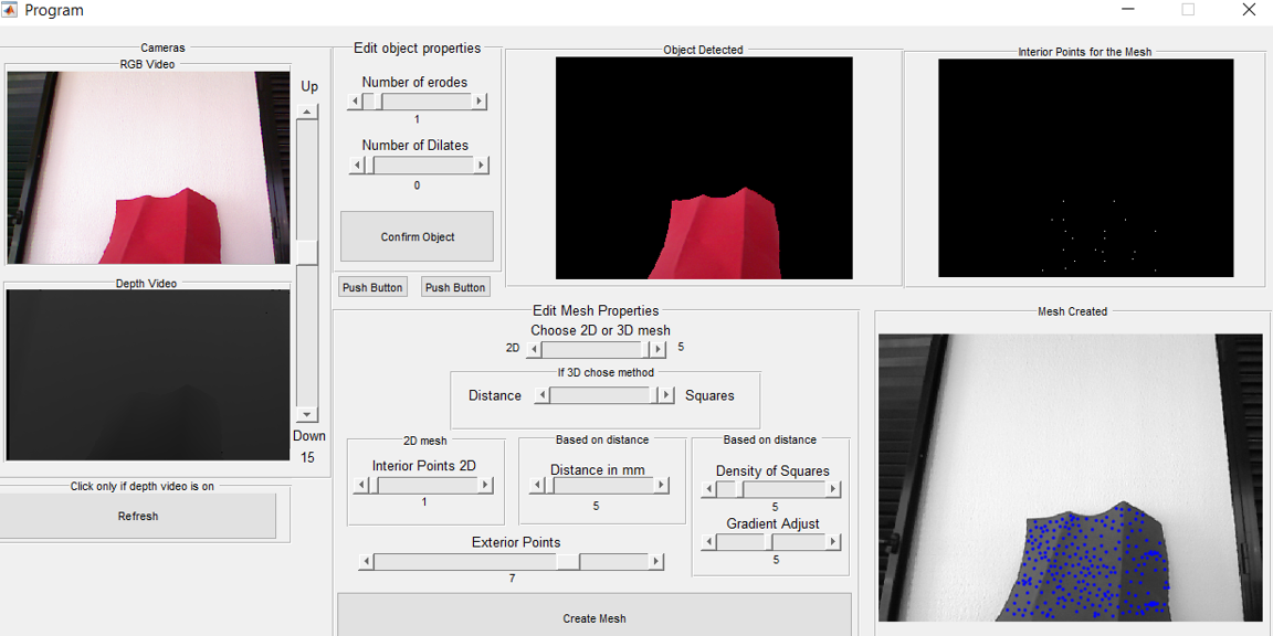 Figure 4 - Mesh using on squares
There are still tests that need to be done on a real object to validate the results.
Also the kinect limitations were study, it was found that minimum distance to the depth sensor to work is 60 cm according to link, but tests with the kinect showed that it can only capture depth if the object is at least at 80 cm.
under construction...
Seventh week
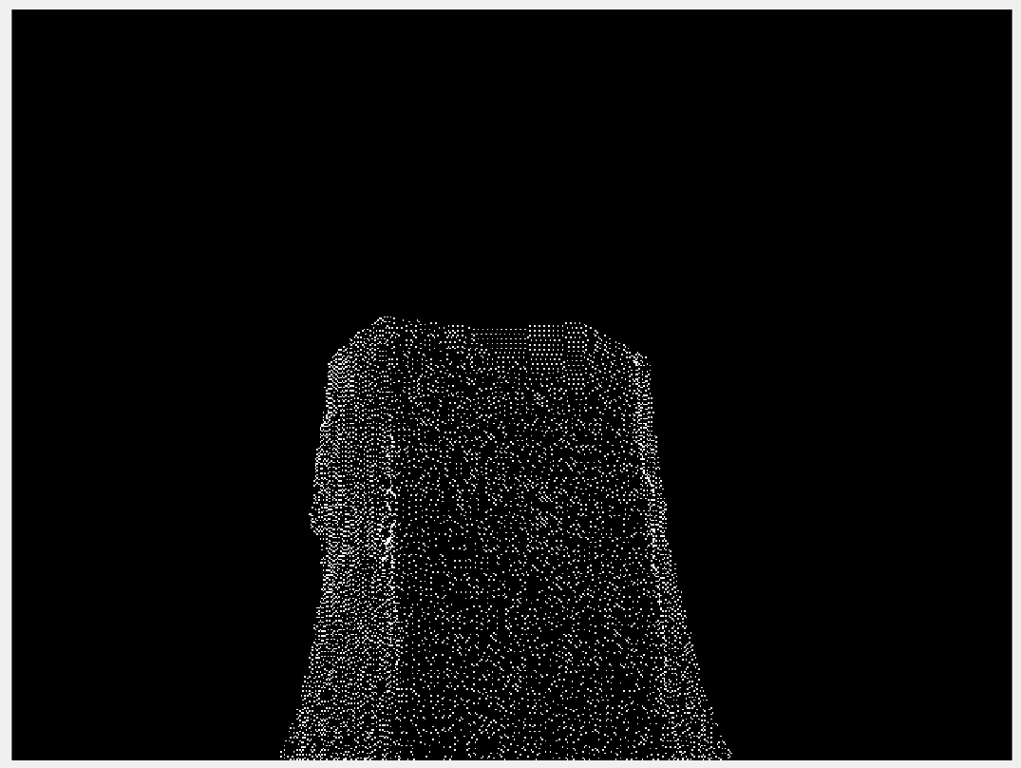
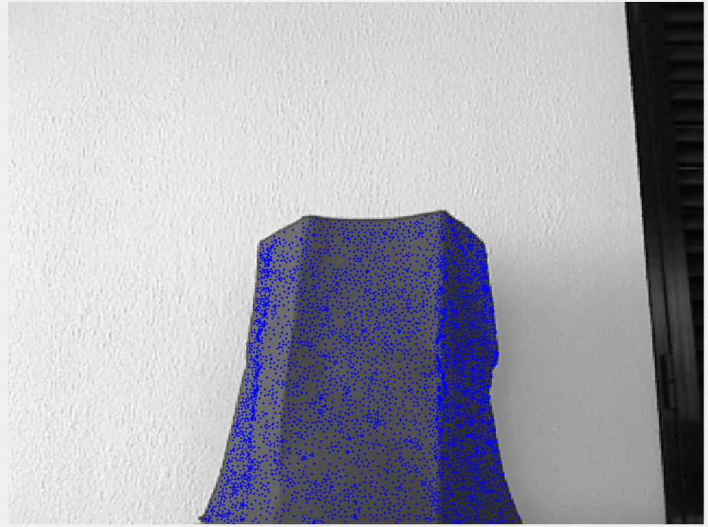
Figure 1- Mesh with 5mm intervals
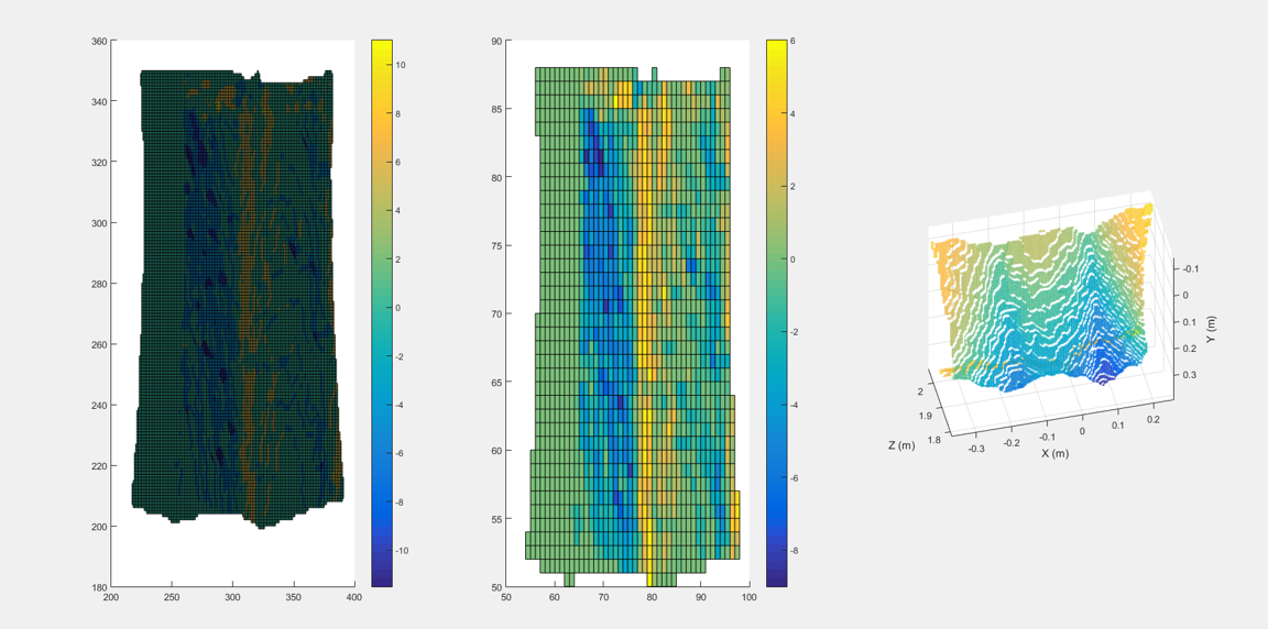
Figure 2 - Division in squares
In figure 2, the gradient from the right object was calculated and the result is the left object, then squares with a stipulated interval were created and the mean gradient in each square was calculated. The result is the middle object.
By using this squares as guide to create the mesh, first a mesh with a certain density was created. This mesh would be to the zone with the highest gradient. Then, from those points, some of then were used in other intervals to create the other meshes densities.
This solution is just for the interior points since the exterior points were calculated the same way as 2D.
By using the delaunay triangulation on those points the result is on figure 3.
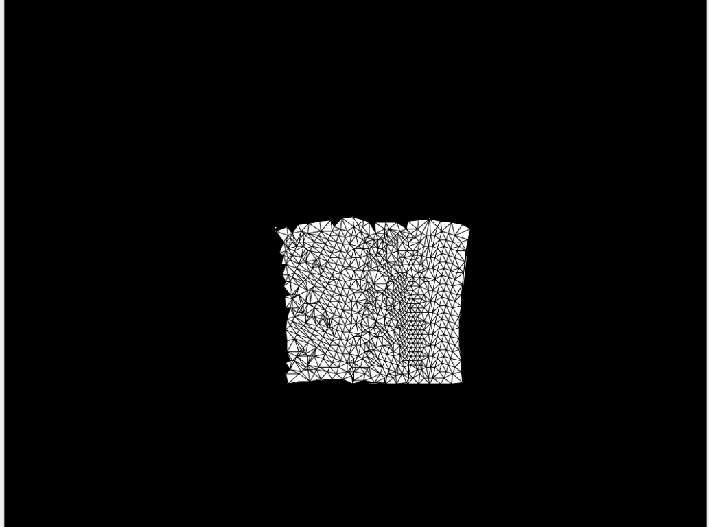
Figure 3 - Mesh for the 3D
This solution does not create a mesh as clean as 2D but the end result is what it was expected. By observing figure 4, it is possible to see that the number of points is higher than the zones with high gradient.
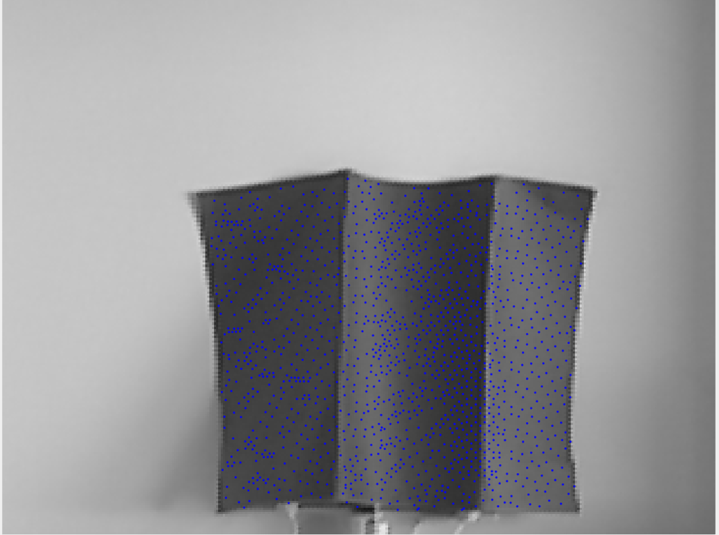
Figure 4 - Result of the process
Another image, closer to the cam allows a better comprehension of the result.
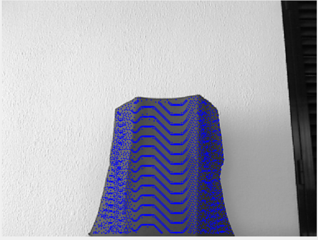
Figure 5 - Result on an object closer to the kinect
Also the drawings for the temporary structure were finished.
Fifth week
The first idea of app is on Figure 1, and for it to work, the imaq.VideoDevice command would be necessary to show the 3D cloud and the cloud gradient but since it was only for show and it's properties could not be changed, both images were removed.
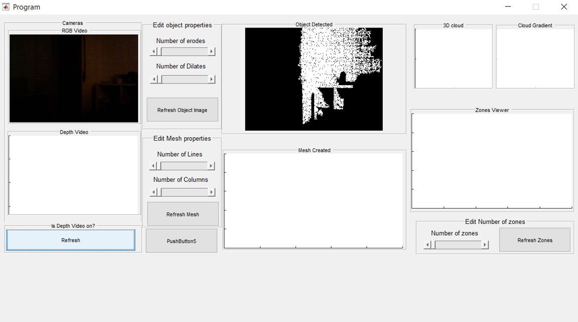
Figure 1 - First stages of the app
Since it would need a way to connect to the arduino, send the mesh coordinates and do the necessary calibrations, more buttons would need to be added on the future.
It was also found a way to control the height of the camera. It was found that it only works when it is used to set the depth camera properties, since doing it on the RGB camera would result in an error.
By using the app, it was noticed that the control of zones was giving bad results. The figure 2 was made using surf command, so it does not show the gradient between height, it shows yellow colour represents the highest height and the blue the lowest.
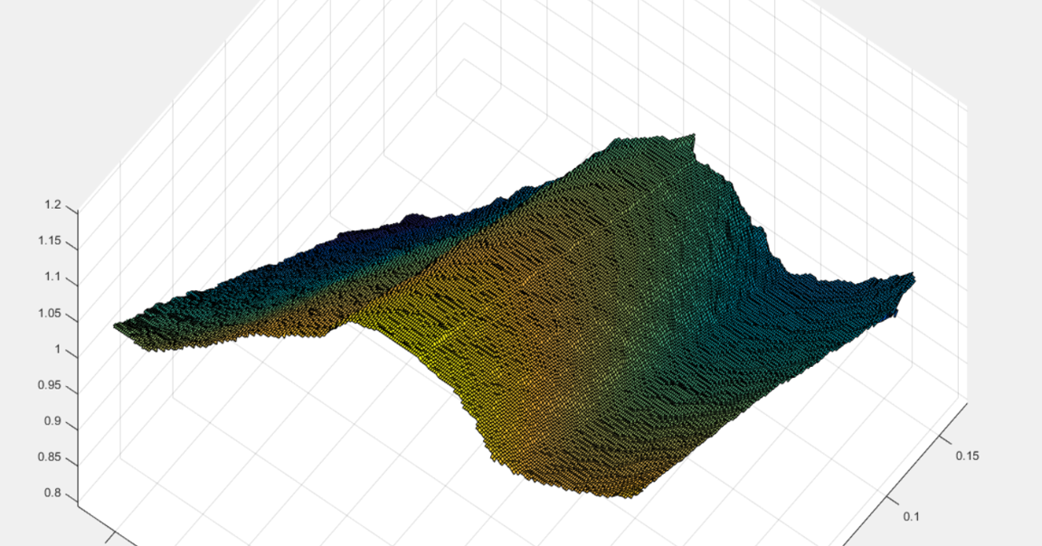
Figure 2 - Zones.
The problem with the gradient was that even thou the surface shape could be seen in figure 2 very well, the result of the function gradient is on figure 3.
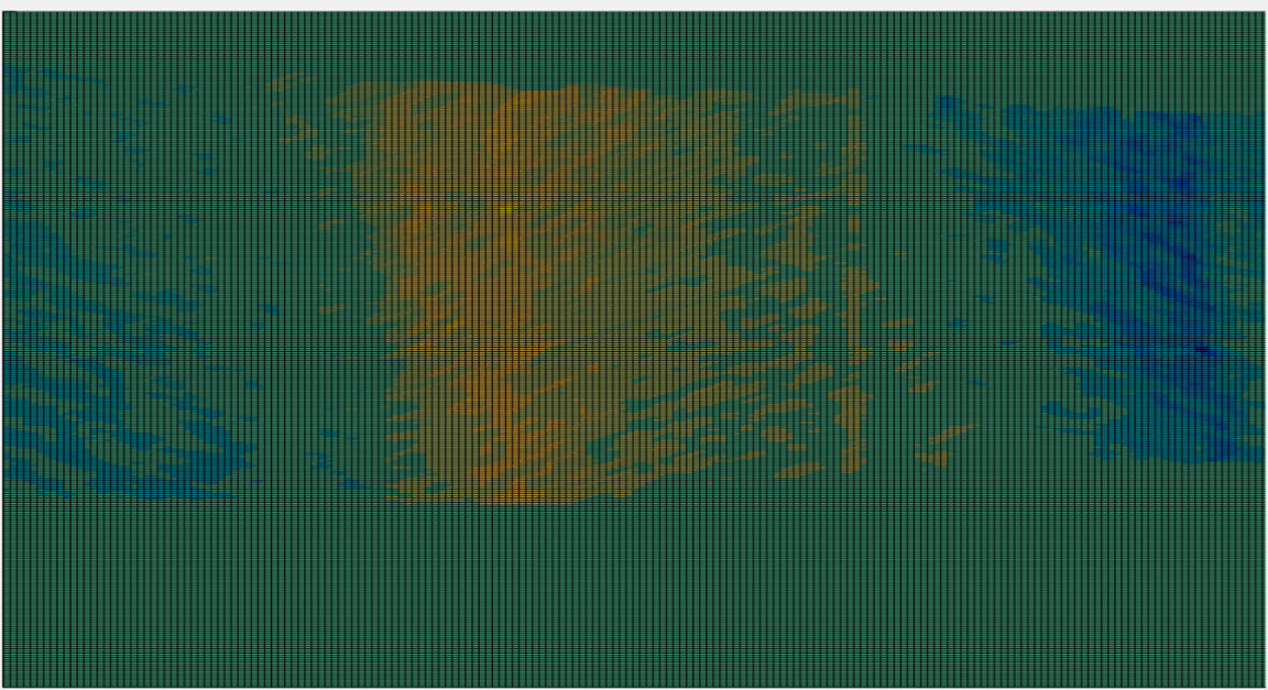 Figure 3 - Gradient function
With these results, the first idea to separate the image based on its gradient, and then threat each zone as an object would work but it would take a lot of time to calculate and the result, possibly would not be as expected.
Also, the mesh processing was now done using exterior points based on the canny filter and the result was better.
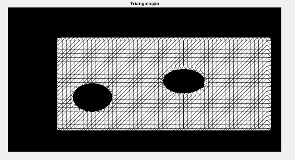 Figure 4 - Mesh using canny to find the contours
By testing it on the app, it was found that the result it produced were much cleaner on the contours than the function used before, but, it is just in 2D.
Fourth week
In this week, it is expected that the image and 3D cloud treatments are finished. First it was necessary to remove the noise from the depth sensor from the kinect like the next example. 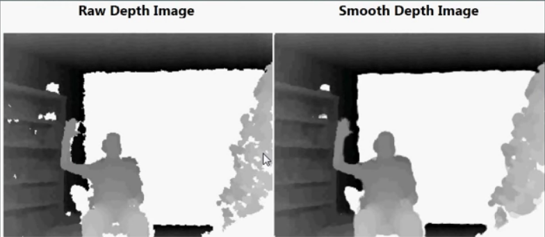
Image 1- example of a 3D image smoothing
To do so, first it was tried a function available at Link
The use of this function created another problem, some of the information was deleted.
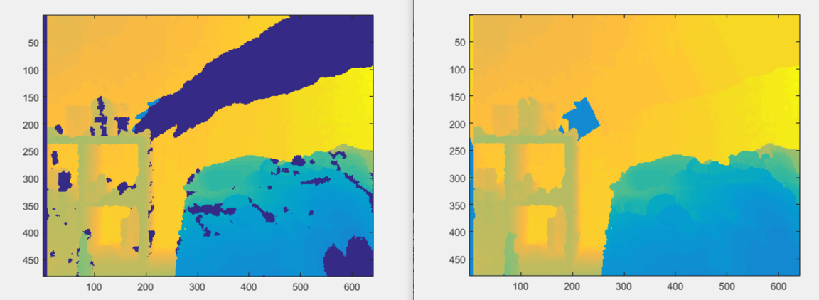
Figure 2 - Funcion kinect depth normalization
As it is possible to see on figure 2, my arm disappear in the right image as well as most of the detail. This would possible create problems by not detecting the holes on a surface or maybe confuse a surface with the background.
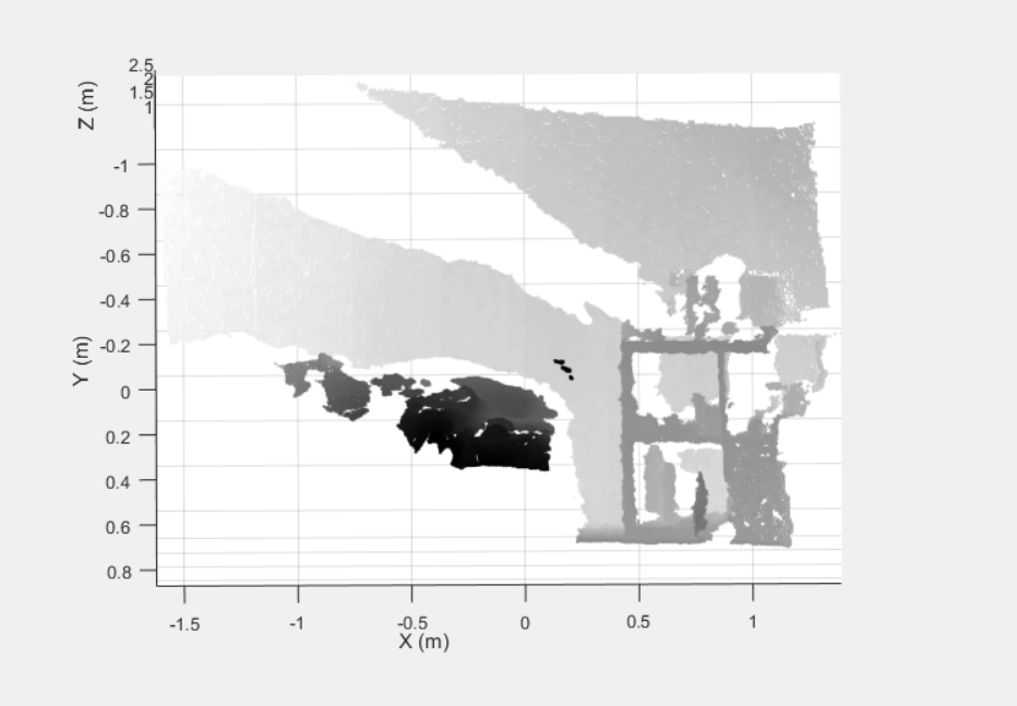
Figure 3 - Point Cloud with kinect depth normalization
As it is possible to see in figure 3, the point cloud is missing a lot of detail, almost the same as if it was not used.
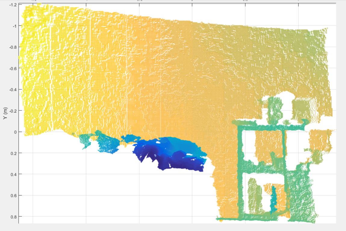
Figure 4 - Original Point cloud
The original point cloud was obtained using the tutorial that was available at mathworks at 06/03/2017 on the Link
Since the function created more problems than those it could solve, another solution was attempted. By observing the preview image of the depth video feed from the kinect, it was noticed that parts of the image would appear and disappear with time. So the solution tried was to get multiple snapshots and complete the missing information in one snapshot with the others.
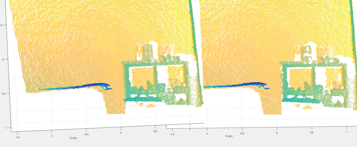 Figure 5 - Comparison between the original mesh (right) and the mesh with multiple layer (left)
As it is possible to see, the mesh on the left is more refined than the one on the right, the only inconvenient is that it takes a couple of seconds to get all the snapshots. The method used to get all the snapshot was a for cycle with a pause of some milliseconds between each, then a mask was created to read all values of 0 from the previous snapshot and replace them with values from the new if available. The replacement was done by multiplying the mask by the new snapshot. The mask was from type uint16 as well as the snapshot.
Now with the refined mesh, it is necessary to associate the depth coordinates with the 2D from the image.
The firs thing done was to remove all of the points that would not be from the intended part. This was done with the same method described before, using a mask and multiplying operations. The result is in figure 6.
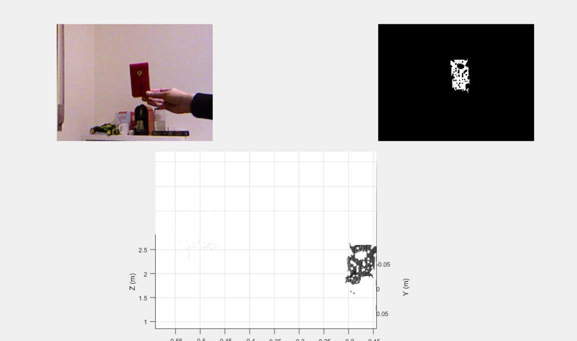 Figure 6 - Mesh treated
This was just to test the concept, so the mesh and the image with the black background, in figure 6, did not received any complex treatment, just a conversion from RGB to HSV and then the values of the H from the powerbank were chosen by trial an error.
To test it on a more controlled environment, a scene was created to simulate possible working conditions.
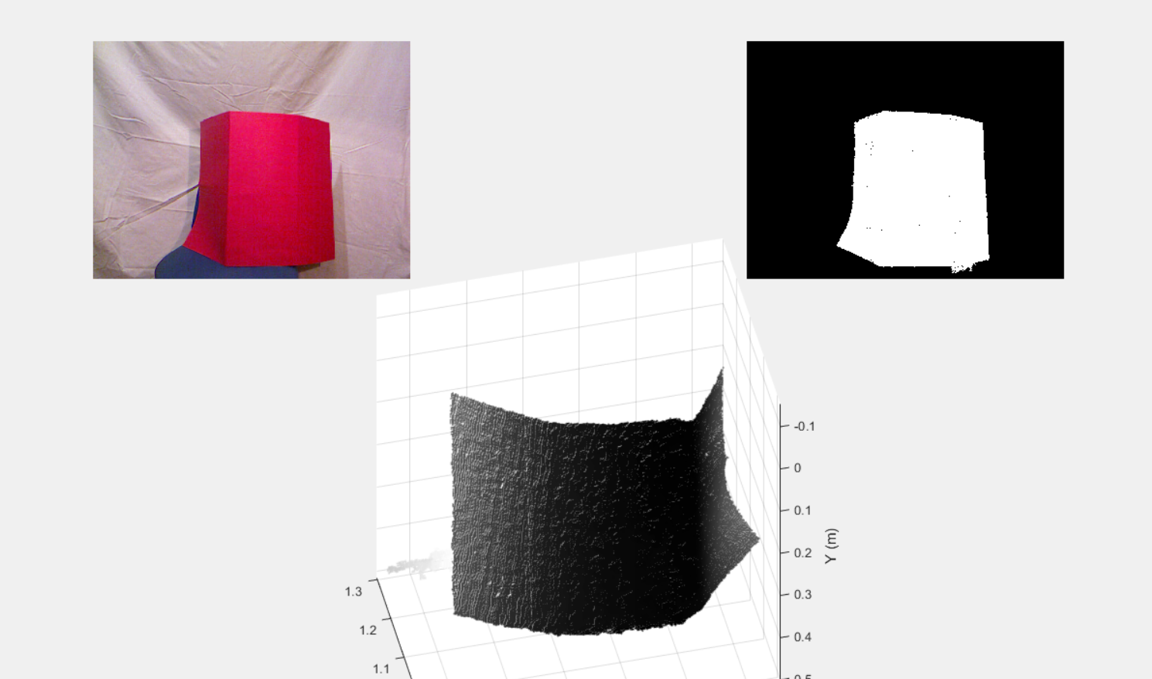 Figure 7 - Test on a "controlled environment"
In this test its possible to see the surface is much more refined, as the previous it was very hard to get the same result and it would influence the gradient calculations.
Now with this surface, the gradient was calculated so it would be possible to divide the surface in zones with same intervals of gradient. The result is in the following image.
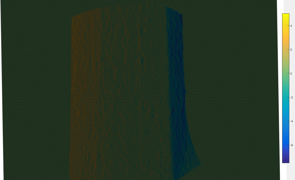
Figure 8 - Gradient calculations
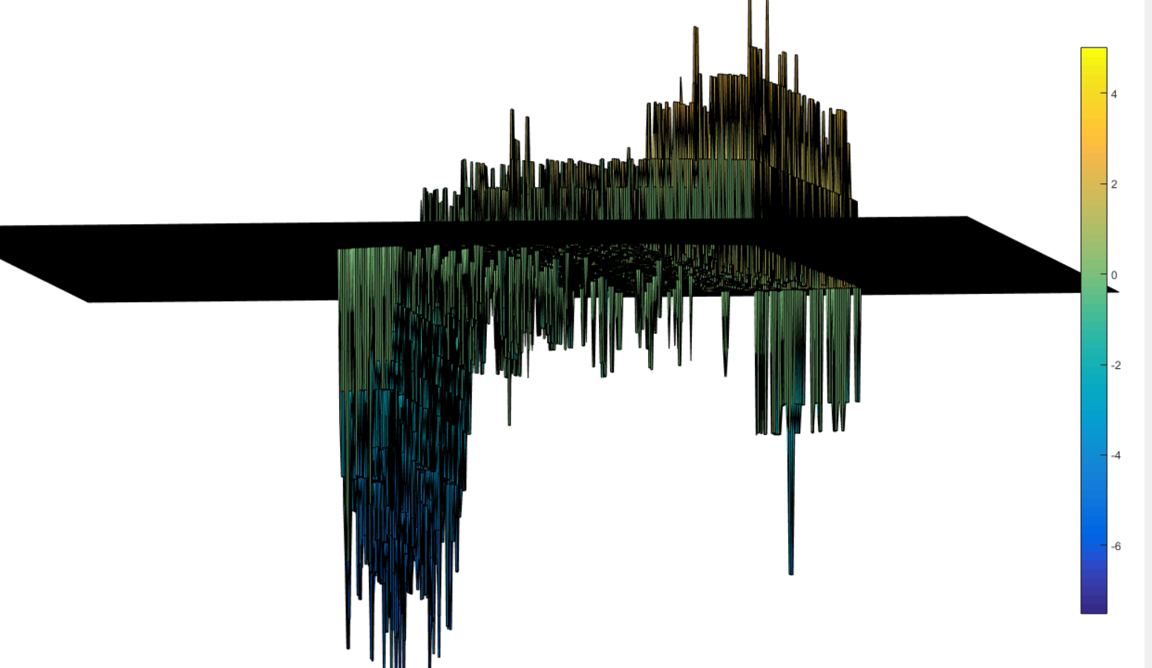
Figure 9 - Gradient Bars
As it can be seen on both images, 3 zones can be visualized. Also an median filter was used to smooth the values.
Now it is just necessary the creation on zones based on the different gradients calculated.
The idea was to use the max and min values from figure 9 and divide into a certain number of similar intervals. The first trial resulted in the figure 10.
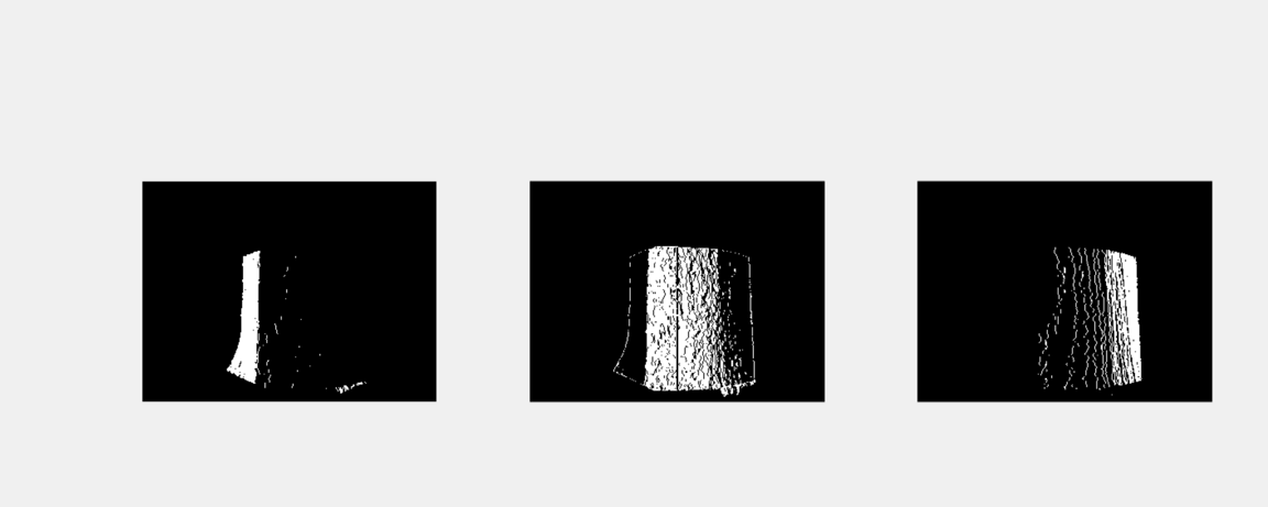 Figure 10 - Different zones
The different zones still would need treatment but it would be interesting to first developed a user interface that could change different parameters in order to get the expected results.
Third Week
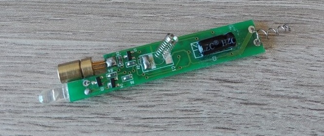 Figure 1 - Laser pointer
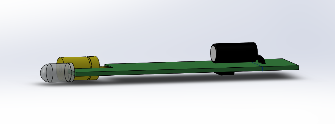
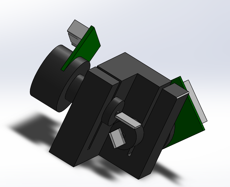
Figure 2 - 3D modelled laser pointer
Since there is still the need to find a system of mirrors to allow the laser pointer and the laser from the vibrometer to be reflected to the galavanometer, a temporary structure was created to facilitate the use of the devices.
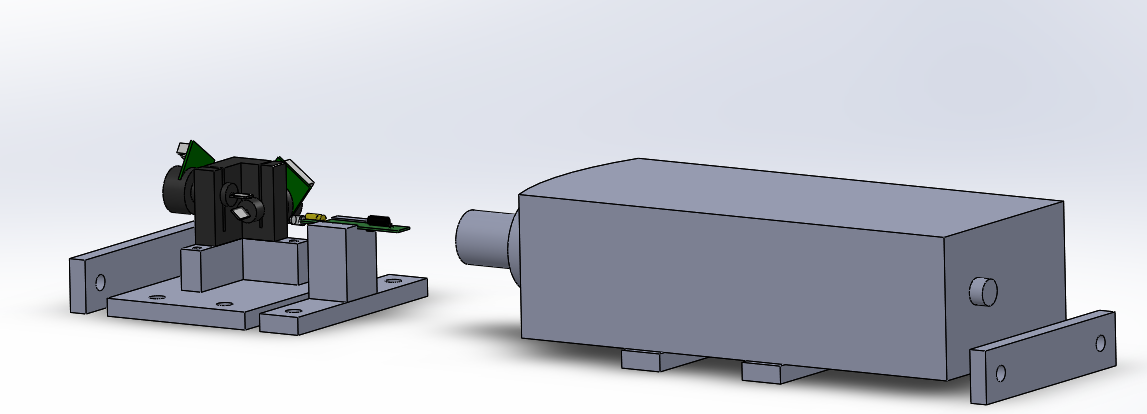
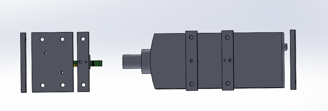
Figure 3 - 3D model of the temporary structure
Second week
Anyway, the galvanometer arrived and all it's components.
All the components were 3D drawed using Solidworks.
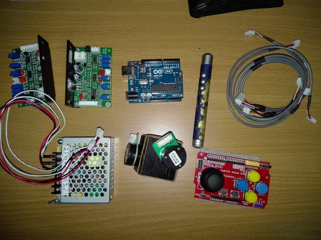 Figure 1 - Material to be used on the work
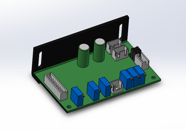
Figure 2 - 3D representation of the galvanometer drivers
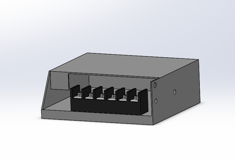
Figure 3 - 3D representation of the galvanometer power source
Then a box that would contain the components was also thought and drawed.
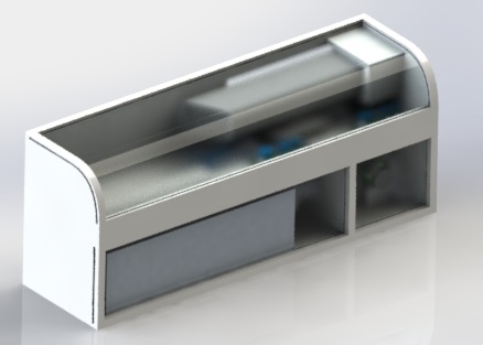
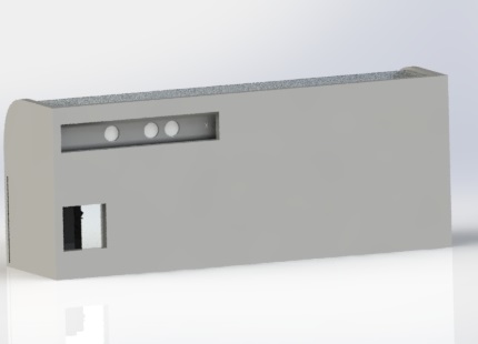 Figures 5 and 6 - 3D representation of the gadget box
As for the mesh creation program developed on matlab, a new aproach was made. Now the mesh is created, on the vertices of the image and then, Delaunay triangulation was made using points gathered inside the surface boundaries and the vertices found calculated.
The result is represented on the next figure.
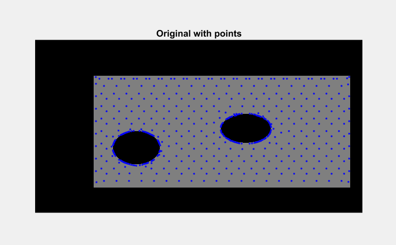
This approach allows to use 3D data gathered from the kinect, (3D point cloud) and use it's points to create the mesh. Then the points that would be sent to the galvanometer, would be the centroid of each triangle. There is still the need to remove the excessive points on the vertices.
Now it is just necessary to get the 3D point cloud from the kinect, build the box for the content and program the arduino.
First week
For the beginning some images created using paint were used to simulate the objects that would be expected the future.
The first image was a rectangle with two wholes.
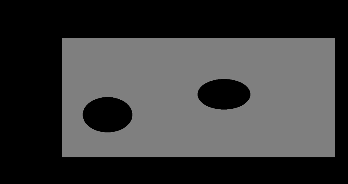 Figure 2 - First image used
This image was converted to gray levels and binarized resulting in a black and white image.
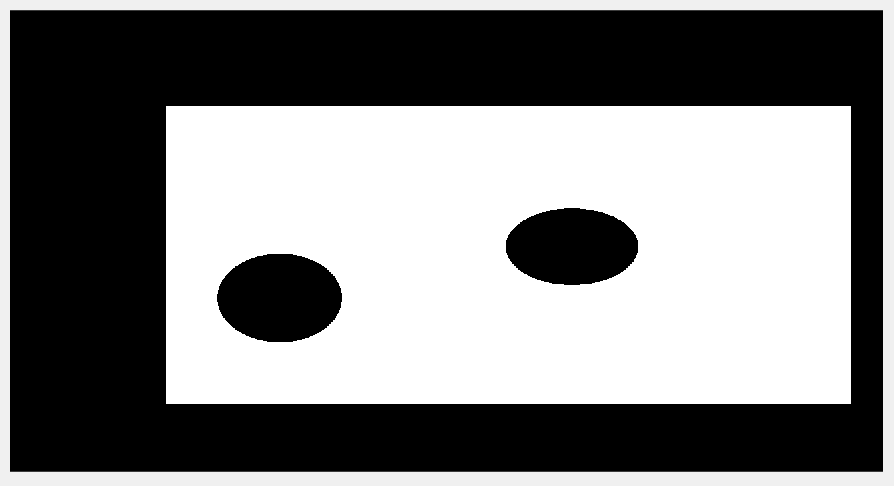 Figure 3 - Binarized image
After getting the image binarized, the object with the biggest area was selected, in this case since there is only one object it is not possible to see the effect. This selection was used to remove possible image nose that could be encounter in an image from the kinect cam.
With only the intended object selected, a mesh was created. First all the pixels from the image were read. Then only the pixels with value one, (pixels that correspond to the location of the object), were selected as valid for the mesh. At last, for cycle was used to select only a few of the valid points of the previous step.
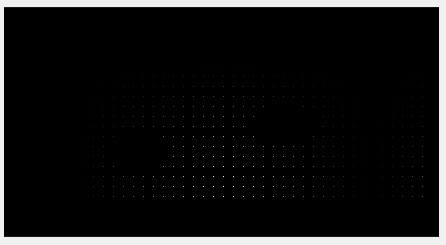 Figure 4 - Mesh created
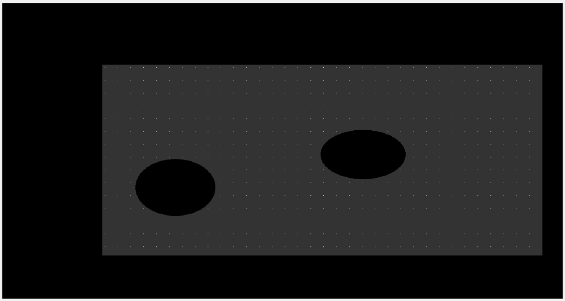 Figure 5 - Representation of the mesh above the surface
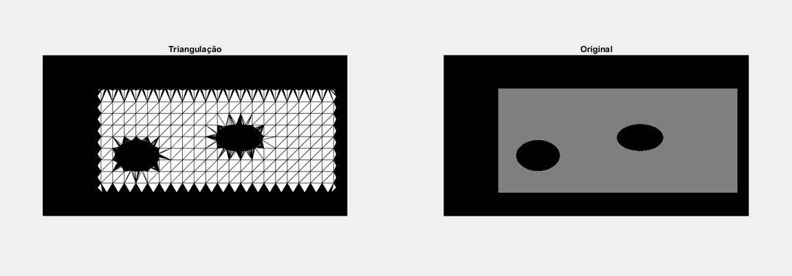
Another representation of the mesh were tried using delaunay triangulation but it was hard to control and took more time to compute. The end result is displayed on the next image.
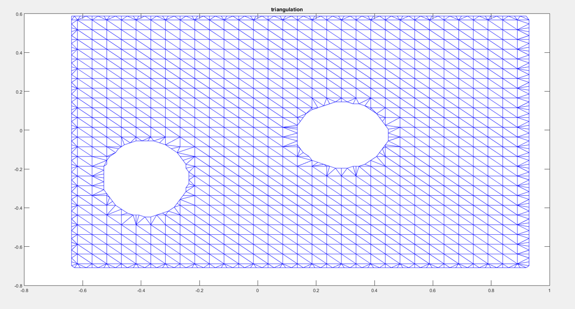
Figure 6 - Mesh using delaunay triangulation
The code used to create this mesh was found at Link
From the images tested, it was reached the conclusion that they needed to be squared and the mesh density would increase or decrease with their dimensions. So the